Measurement of Capacitance By Schering Bridge:
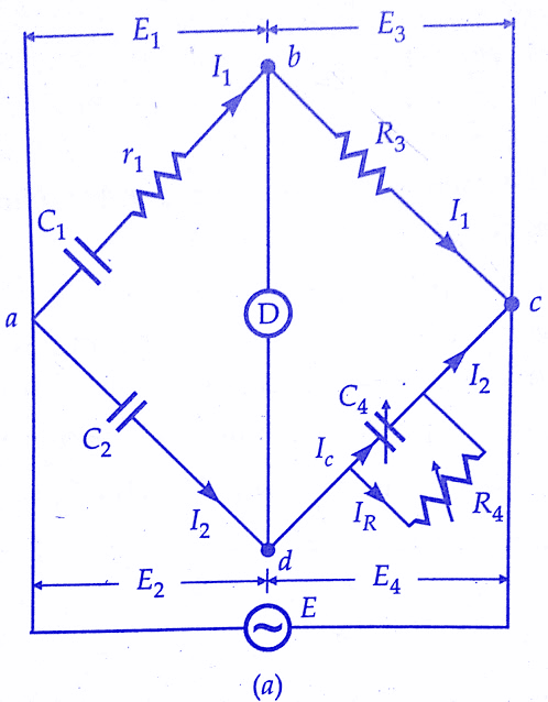
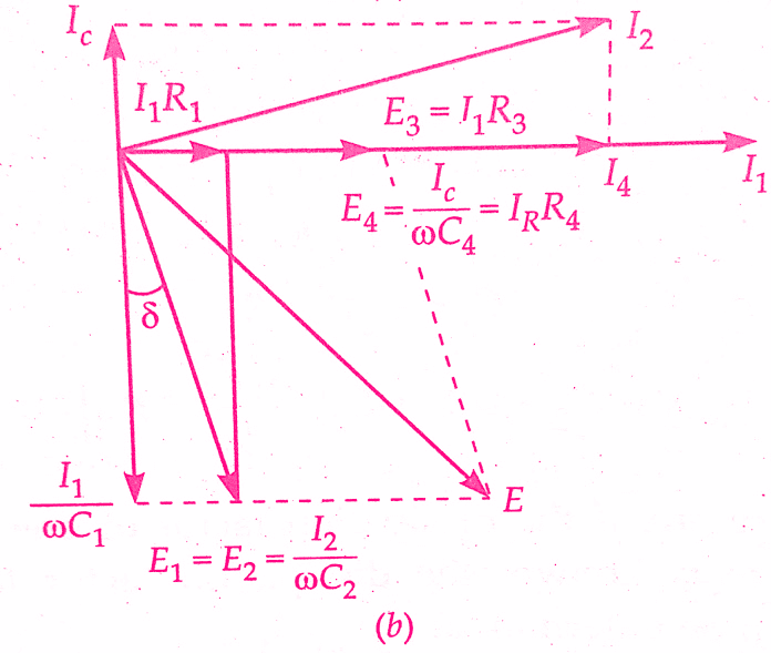
We will discuss the measurement of capacitance by Schering bridge. The connection and phasor diagram of Schering Bridge under balance conditions are shown in the below figure.
In the realm of electrical engineering and circuit analysis, the accurate measurement of capacitance is of utmost importance. Capacitors, vital components in numerous electronic devices, store electrical energy and play a pivotal role in various applications such as signal filtering, energy storage, and timing circuits.
One widely-used method for measuring capacitance with high precision is the Schering Bridge, a balanced bridge circuit that exploits the principles of impedance to yield accurate capacitance readings. In this article, we will delve into the Schering Bridge, understanding its working principles, components, and the steps involved in capacitance measurement.
The Schering Bridge, also known as the Maxwell-Wien Bridge, is a modification of the Wheatstone Bridge configuration, tailored specifically for measuring the capacitance of a capacitor. Just like the Wheatstone Bridge is designed for measuring resistances, the Schering Bridge serves as an invaluable tool for accurate and reliable capacitance measurement.
Components of the Schering Bridge:
- Capacitor Under Test (CuT): The capacitor whose capacitance is to be measured is connected to one arm of the bridge.
- Standard Capacitor (Cs): A known and calibrated capacitor is connected to another arm of the bridge.
- Variable Resistance (Rv): A variable resistor is connected in parallel with the standard capacitor to ensure balance in the bridge.
- Variable Capacitor (Cv): A variable capacitor is connected in parallel with the capacitor under test.
Working Principle:
The Schering Bridge operates on the principle of impedance matching, where the bridge becomes balanced when the impedance of the arms containing the standard capacitor and the variable resistor matches the impedance of the arms containing the capacitor under test and the variable capacitor.
When the bridge is balanced, the phase difference between the voltage across the arms is zero, indicating that the impedance ratios are equal. This balance condition is achieved by adjusting the variable resistor and capacitor in such a way that the bridge becomes insensitive to the frequency of the applied AC voltage.
Steps Involved in Capacitance Measurement:
- Initial Setup: Connect the capacitor under test (CuT) and the standard capacitor (Cs) to their respective arms of the bridge. Make sure the variable resistor (Rv) and the variable capacitor (Cv) are initially set to a known value.
- Applying AC Voltage: Apply an AC voltage of a known frequency to the bridge circuit.
- Adjusting Components: Begin by adjusting the variable resistor (Rv) until the bridge becomes balanced. This is typically done by observing the null point on an oscilloscope or a null detector.
- Fine-tuning with Variable Capacitor: After balancing the bridge with the variable resistor, fine-tune the bridge by adjusting the variable capacitor (Cv) until the bridge is balanced again. This indicates that the impedance ratio of the two arms is matched.
- Capacitance Calculation: Once the bridge is balanced, the capacitance of the capacitor under test can be calculated using the formula:
CuT=Cs(Rref/Rv)8(Cref/Cv)
Where Cs is the value of the standard capacitor, Rv is the value of the variable resistor at balance, Rref is a reference resistance, Cv is the value of the variable capacitor at balance, and Cref is a reference capacitance.
Advantages of the Schering Bridge:
- High Accuracy: The Schering Bridge offers a high degree of accuracy in capacitance measurement, making it suitable for applications where precision is essential.
- Frequency Insensitivity: This bridge configuration is designed to be insensitive to the frequency of the applied AC voltage, ensuring consistent measurements across different frequency ranges.
- Calibration Capability: By using a known standard capacitor, the Schering Bridge can be calibrated, enhancing the reliability of measurements.
Let
C1 = capacitor whose capacitance is to be determined,
r1 = a series resistance representing the loss in the capacitor
C2 = a standard capacitor.This capacitor is either an air or a gas capacitor and hence is loss-free.However, if necessary, a correction may be made for the loss angle of this capacitor,
R3 = a non-inductive resistance,
C4 = a variable capacitor, and
R4 = a variable non-inductive resistance in parallel with variable capacitor C4.
Must Read:
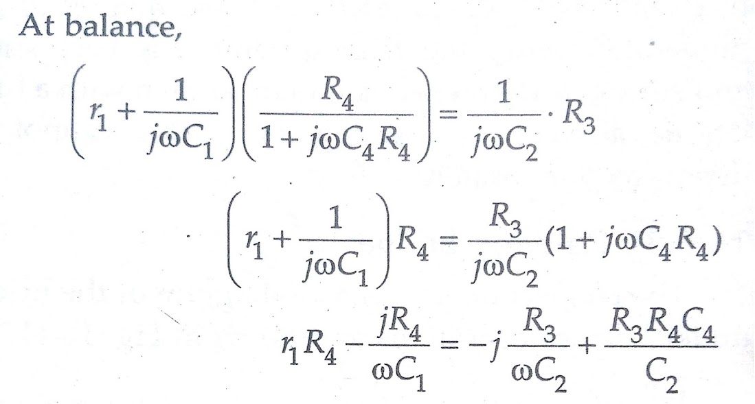
Equating the real and imaginary terms, we obtain
r1 = R3C4/C2
and C1 = C2 ( R4/R3)
Two independent balance equations are obtained if C4 and R4 are chosen as the variable elements.
Must Read:
Measurement of dissipation factor by Schering Bridge:
Dissipation factor,
D1 = tan δ = ωC1r1 =ω(C2R4/R3) x (R3C4/C2) = ωC4R4
Therefore values of capacitance C1, and its dissipation factor are obtained from the values of bridge elements at balance.
Permanently set up Schering bridges are sometimes arranged so that balancing is done by adjustment of R2 and C4 with C2 and R4 remaining fixed. Since R3 appears in both the balance equations and therefore there is some difficulty in obtaining balance but Schering Bridge has certain advantages as explained below :
The equation for capacitance is C1 = (R4/R3) C2 and since R4 and C2 are fixed, the dial of resistor R3 may be calibrated to read the capacitance directly.
Dissipation factor D1 = ωC4R4 and in case the frequency is fixed the dial of capacitor C4 can be calibrated to read the dissipation factor directly.
Let us say that the working frequency is 50 Hz and the value of R4 is kept fixed at 3,180 Ω.
Dissipation factor,
D1 = 2π x 50 x 3180 x C4 = C4 X 10⁶.
Since C4 is a variable decade capacitance box, its setting in μF directly gives the value of the dissipation factor.
It should, however, be understood that the calibration for dissipation factor holds good for one-particular frequency, but may be used at another frequency if correction is made by multiplying by the ratio of frequencies.
Must Read:
Conclusion:
In this, we have learnt Measurement of Capacitance & dissipation factor by Schering Bridge. You can download this article as pdf, ppt.
Comment below if you have any queries!
thanks